I wrote a post about this paper a year ago – embarrassingly, it appears I never pressed “Publish”. I’ve updated it for you too.

One of the current challenges in space weather modelling is to capture the variety of observations in our physical models. In meteorology, one such technique is ensemble modelling – we applied this to simple radiation belt models, to build a foundation for future ensembles in forecasting. Our paper “Two methods to analyze radial diffusion ensembles: The perils of space- and time-dependent diffusion” was published in Physics of Plasmas as a Featured Article. This 4+ year journey led us to new techniques and to several unexpected and intriguing results that throw up some questions about everyday choices in radiation belt diffusion modelling. These mainly arise because we are modelling in the $L^*$ domain… and the amount of diffusion varies as $L^*$ varies.

Our two key results explained here:

• Both the location / distance of the outer boundary, and the outer boundary condition change the way in which the system evolves – but there is no clear “most physical” choice. Observations can help limit this for hindcasting, but… what should we use?
• In our experiments, the gradient of the phase space density ($PSD$) contributed more to the evolution of the system, rather than the diffusion coefficient $D_{LL}$. If true, should we focus on determining the $PSD$ than on $D_{LL}$? If it’s not true, are 1d-radial diffusion models inappropriate radiation belt toy models?

The model

In radiation belt modelling, we can approximate belt evolution by considering diffusion across three adiabatic invariants of magnetically trapped particles. The third invariant (magnetic flux enclosed on a drift path around the Earth) is much longer than the other timescales and can be modelled by itself as an approximation of the belts. We use a Fokker-Planck model,

where f is the phase space density, $L^*$ is related to the third adiabatic invariant and as a rough guide can be considered “how far the drift path is from the Earth, in Earth radii”, $D_{LL} = D_0L^*$ is the diffusion coefficient and $\mathcal{L}$ incorporates loss.

Major results

New tools to measure the difference between ensemble members

We can’t compare model results to any ground truth; nevertheless, in any radiation belt model a variety of metrics are used to compare a variety of outputs. We found that:

The shape of the distribution is a useful and representative measure

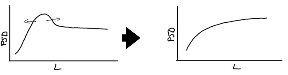
We found that any threshold-based methods to find when the simulation was “done” (e.g. these two distributions are the same when mean square error is less than X) were completely dependent on the (arbitrary!) choice of threshold. Instead, we chose a measure of the diffusion that represents what we’re often interested in – how long for radial diffusion to reduce an enhancement by diffusing it away (“time to monotonicity“)

There are extremely useful analytic approaches we have never used

The second metrics we used were analytic: the mass- and energy-like density

$\mathcal{N}$ clearly represents the total mass in our simulation at a given time step. $\mathcal{E}$ is more interesting; it represents how far we are from a low-energy or equilibrium state. We use it to quantify how the system evolves towards equilibrium.

New insights about the boundary

It’s long been understood that the outer boundary of radiation belt models is important but tricky: we only have data far inside the true boundary, which is difficult to define and difficult to find in observations. An additional question we had going in was “What about the $L^*$ dependence of diffusion?” Many models in practice are cut short to a domain where data can constrain them. But if the amount of diffusion depends on where we are in $L^*$, what does that imply about our abbreviated models?

Outer boundary conditions used currently are not physical

We tested both Neumann (fixed gradient; the radiation belt continues past the model domain) and Dirichlet (fixed value; say that data is available to constrain it) outer boundaries. Both essentially impose unphysical results.

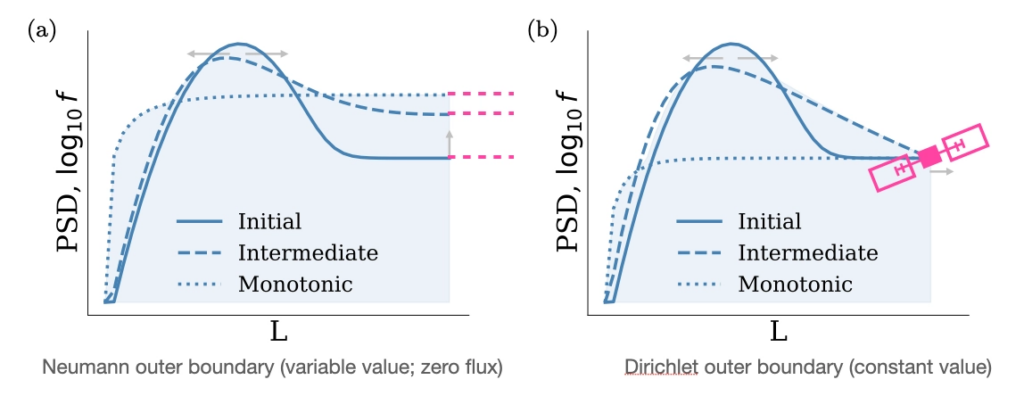
With a Neumann outer boundary the injection diffuses away quickly because the particles can move outwards and the phase space density at the outer limit can rise – but this represents a large increase outside the domain. With a Dirichlet outer boundary, this cannot happen, but nor can material flow outwards. In our experiments we found that far more ensemble members with a Neumann outer boundary reached monotonicity (where the injection diffused away) Recent work has shown that data-derived Dirichlet models which are most common are indeed the best current compromise (Lee et al., 2024) but these will not work when forecasting, as such data is obviously not yet available. Mixed boundary conditions will be more physical to represent the continuation of material outside the modelled domain.

Cutting short the domain changes the physics

The amount of diffusion that occurs is dependent on where we are within the domain; it depends on $L^*$. The rate of diffusion at $L^*=6$ will be higher than at $L^*=4$; more material is lost when the domain is longer. However, domain length also interacts with the type of boundary condition.

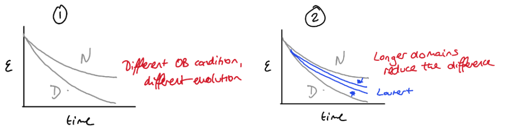
The doodles above summarise this: the energy-like quantity $\mathcal{E}$ which represents how far we are from equilibrium is different for Neumann vs Dirichlet conditions, but the longer the domain, the more similar they become.

Should we spend time improving the diffusion coefficient $D_{LL}$ or the phase space density $PSD$?

Using an analytic tool such as $\mathcal{E}$ allows us to compare the relative contribution of different model components to the resulting diffusion by considering $\mathcal{E}_t$. We find that:

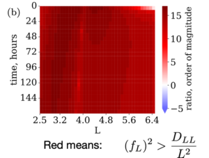
You’ll notice that this is all red. This means that across the model domain, the gradient of the phase space density contributes more to the evolution of the particle distribution than the diffusion coefficient $D_{LL}$. This directly contradicts current practice in radiation belt modelling, where the focus is on developing appropriate $D_{LL}$.

How significant would this be in a less idealised scenario?

Obviously this is a very simple model, but we need to understand how model changes affect the final ensemble. Changes in the initial phase space density and in the outer boundary location are actually (in general) dominated by loss processes, once we add them in – although if the plasmasphere causes loss at high $L^*$ than a simple monotonic distribution is never reached. Nevertheless, boundary conditions and location still need to be more physical when we don’t have data to constrain them – i.e. for forecasting and nowcasting.

The results comparing relative contributions from $D_{LL}$ and $PSD$ is concerning. Is this an indicator suggesting a shift of focus? Conversations with modellers of the full radiation belts suggest that this is not what they see in practice. Perhaps this model is too idealised? We need to test this further.

And to answer my original question, “What are realistic radial diffusion timescales for an injection?”: From hours to a week. Very helpful.

Links:

• The paper can be found at https://doi.org/10.1063/5.0217268
• A Python notebook to make figures shown in the paper can be found at https://zenodo.org/doi/10.5281/zenodo.13336681
• I presented this at a MIST seminar and at a Physics of Plasmas webinar, both of which can be watched online.